Reading and Writing Memory in Different Halves of the Cycle

Arrangement of Computer Systems:
§ five: Pipelining

Instructor: M.S. Schmalz

Reading Assignments and Exercises

This section is organized as follows:

5.1. Overview of Pipelining
5.ii. Pipeline Datapath Pattern and Implementation
v.3. Pipeline Control and Hazards
5.4. Pipeline Performance Analysis

Information contained herein was compiled from a variety of text- and Web-based sources, is intended as a teaching aid only (to be used in conjunction with the required text, and is not to exist used for any commercial purpose. Particular cheers is given to Dr. Enrique Mafla for his permission to use selected illustrations from his course notes in these Web pages.

5.1. Overview of Pipelining

Reading Assignments and Exercises

Call up that, in Section iv, nosotros designed a multicycle datapath based on (a) edifice blocks such equally multiplexers for selecting an functioning to produce ALU output, (b) ALUs to compute addresses and arithmetic or logical operations, and (c) components such as memories or registers for long- or short-term storage of operands or results. Nosotros also showed that the multicycle datapath is, in exercise, more efficient than the unmarried-cycle datapath.

In this section, we continue our quest for efficient ciphering by discovering that we can overlay single-cycle datapaths in fourth dimension to produce a type of computational architecture chosen pipelining. Nosotros prove that pipelined architectures, when they work properly and are relatively complimentary from errors and hazards such as dependencies, stalls, or exceptions can outperform a simple multicycle datapath. Likewise, we discuss bug associated with pipelining that limits its usefulness in various types of computations.

5.1.1. Concept of Pipelining

Suppose yous wanted to make an automobile from scratch. You might assemble up the raw materials, form the metal into recognizeable shapes, cast some of the metallic into an engine block, connect up fuel lines, wires, etc., to eventually (one would promise) brand a workable automobile. To do this, you would need many skills - all the skills of the artisans that brand autos, and management skills in addition to existence an electrician and a metallurgist. This would non be an efficient way to brand a car, but would definitely provide many challenges.

That is the way a multicycle datapath works - it is designed to do everything - input, output, and computation (recall the fetch-decode-execute sequence). We need to enquire ourselves if this is really the best way to compute efficiently, specially when nosotros consider the complication of control for big (CISC) systems or even smaller RISC processors.

Fortunately, our analogy with car-making is non so far-fetched, and tin can actually help u.s.a. go far at a more efficient processor design. Consider the modernistic way of making cars - on an assembly line. Here, in that location is an orderly flow of parts down a conveyor belt, and the parts are processed by unlike stations (also called segments of the assembly line). Each segment does i affair, over and over. The segments are coordinated to exploit the sequentiality inherent in the automobile assembly process. The piece of work gets done more smoothly (because of the orderly flow of input parts and output results), more efficiently (because each assembler at each segment of the pipeline does his or her task at what one hopes is maximum efficiency), and more than reliably considering there is greater consistency in one task being done repetitively (provided the assembly line is designed correctly).

A similar illustration exists for computers. Instead of a multicycle datapath with its complex control arrangement that walks, talks, cries, and computes - let us suppose that nosotros could build an associates line for calculating. Such objects really exist, and they are called pipeline processors. They have sequentially-arranged stages or segments, each of which perform a specific job in a fixed corporeality of time. Information flows through these pipelines like cars through an assembly line.

v.1.2. Definitions and Practical Observations well-nigh Pipelines

We next consider several terms and some practical bug associated with pipeline processors.

5.1.2.1. Definition. A pipeline processor is comprised of a sequential, linear listing of segments, where each segment performs 1 computational task or group of tasks.

5.1.2.two. Observation. A pipeline processor can be represented in 2 dimensions, as shown in Figure 5.one. Here, the pipeline segments (Seg #one through Seg #iii) are arranged vertically, so the data tin flow from the input at the meridian left down to the output of the pipeline (after Segment 3). The progress of an instruction is charted in blue typeface, and the next education is shown in cherry-red typeface.

There are 3 things that one must detect virtually the pipeline. Get-go, the work (in a computer, the ISA) is divided up into pieces that more or less fit into the segments alloted for them. 2d, this implies that in order for the pipeline to work efficiently and smoothly, the work partitions must each have about the aforementioned time to complete. Otherwise, the longest partition requiring time T would agree up the pipeline, and every segment would have to take time T to complete its piece of work. For fast segments, this would mean much idle time. Third, in order for the pipeline to work smoothly, there must be few (if any) exceptions or hazards that cause errors or delays within the pipeline. Otherwise, the instruction will have to be reloaded and the pipeline restarted with the aforementioned didactics that causes the exception. There are boosted problems we need to talk over about pipeline processors, which nosotros will consider shortly.

Figure 5.one. Notional diagram of a pipeline processor. The segments are bundled vertically, and time moves along the horizontal centrality.

5.one.2.3. Reponse Time. It is easily verified, through inspection of Figure five.1., that the response time for whatever instruction that takes three segments must be 3 times the response time for any segment, provided that the pipeline was full when the instruction was loaded into the pipeline. Every bit we shall run across later in this section, if an North-segment pipeline is empty before an instruction starts, and then N + (N-1) cycles or segments of the pipeline are required to execute the education, because it takes Northward cycles to make full the pipe.

Notation that we just used the term "bicycle" and "segment" synonomously. In the type of pipelines that we will study in this form (which includes the vast majority of pipeline processors), each segment takes one cycle to complete its work. Thus, an N-segment pipeline takes a minimum time of North cycles to execute one pedagogy. This brings to mind the performance issues discussed in Section v.1.1.five.

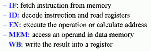
v.1.2.4. Piece of work Sectionalization. In the previous section, nosotros designed a multicycle datapath based on the assumption that computational work associated with the execution of an instruction could be partitioned into a five-step process, as follows:

v.i.2.v. Performance. Considering at that place are Northward segments active in the pipeline at any 1 time (when information technology is full), it is thus possible to execute North segments concurrently in whatever bicycle of the pipeline. In contrast, a purely sequential implementation of the fetch-decode-execute wheel would require Northward cycles for the longest education. Thus, information technology can be said that we have O(Northward) speedup. As we shall meet when nosotros analyze pipeline operation, an exact N-fold speedup does not always occur in practice. However information technology is sufficient to say that the speedup is of order Due north.

5.2. Pipeline Datapath Design and Implementation

Reading Assignments and Exercises

As shown in Section 5.one.2.4, the work involved in an didactics can exist partitioned into steps labelled IF (Pedagogy Fetch), ID (Instruction Decode and data fetch), EX (ALU operations or R-format execution), MEM (Memory operations), and WB (Write-Back to register file). We next discuss how this sequence of steps tin can exist implemented in terms of MIPS instructions.

5.2.1. MIPS Instructions and Pipelining

In order to implement MIPS instructions effectively on a pipeline processor, we must ensure that the instructions are the aforementioned length (simplicity favors regularity) for piece of cake IF and ID, like to the multicycle datapath. We also need to have few simply consequent teaching formats, to avoid deciphering variable formats during IF and ID, which would prohibitively increment pipeline segment complexity for those tasks. Thus, the register indices should be in the aforementioned identify in each instruction. In practice, this means that the rd, rs, and rt fields of the MIPS instruction must not change location across all MIPS pipeline instructions.

Additionally, nosotros want to take instruction decoding and reading of the register contents occur at the same time, which is supported by the datapath architecture that we take designed thus far. Find that nosotros take retentivity address computation in the lw and sw instructions only, and that these are the only instructions in our v-instruction MIPS subset that perform memory operations. Equally before, we presume that operands are aligned in retentivity, for straightforward access.

five.ii.2. Datapath Partitioning for Pipelining

Recall the single-wheel datapath, which can be partitioned (subdivided) into functional units as shown in Figure v.2. Because the single-bicycle datapath contains separate Instruction Memory and Data Retentivity units, this allows us to straight implement in hardware the IF-ID-EX-MEM-WB representation of the MIPS educational activity sequence. Observe that several control lines take been added, for case, to route data from the ALU output (or retentivity output) to the annals file for writing. Also, there are again three ALUs, 1 for ALUop, another for JTA computation, and a 3rd for adding PC+iv to compute the address of the adjacent instruction.

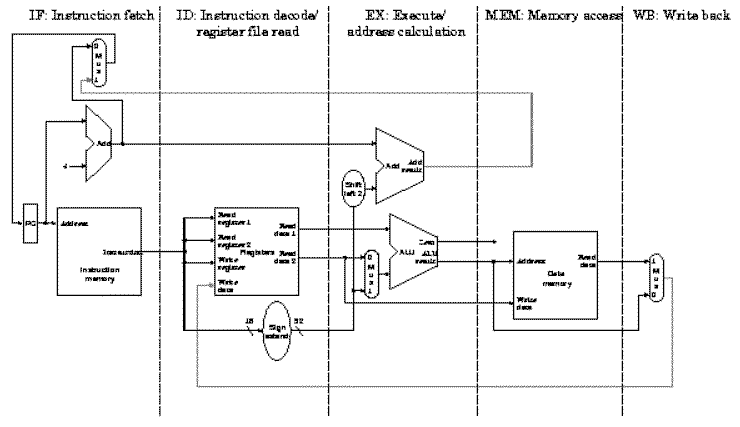
Figure 5.two. Segmentation of the MIPS single-cycle datapath developed previously, to course a pipeline processor. The segments are arranged horizontally, and data flows from left to right [Maf01,MK98].

We can represent this pipeline construction using a infinite-fourth dimension diagram similar to Effigy 5.1, as shown in Figure 5.3. Here iv load instructions are executed sequentially, which are called because the lw instruction is the only i in our MIPS subset that consistently utilizes all five pipeline segments. Observe besides that the right half of the register file is shaded to represent a read operation, while the left half is shaded to represent write.

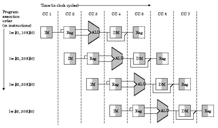
Figure 5.3. Partitioning of the MIPS single-wheel datapath adult previously, with replication in space, to course a pipeline processor that computes four lw instructions. The segments are arranged horizontally, and data flows from left to correct, synchronously with the clock cycles (CC1 through CC7) [Maf01,MK98].

In order to ensure that the single-cycle datapath conforms to the pipeline design constraint of ane bike per segment, we need to add buffers and control between stages, like to the style nosotros added buffers in the multicycle datapath. These buffers and control circuitry are shown in Figure v.4 every bit crimson rectangles, and shop the results of the i-th stage and then that the (i+1)-thursday stage can use these results in the adjacent clock cycle.

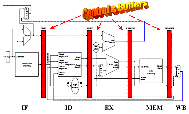
Figure five.four. Addition of control and buffer circuits to Effigy v.3 produces the MIPS pipelined datapath [Maf01,MK98].

In summary, pipelining improves efficiency by showtime regularizing the instruction format, for simplicity. We then divide the instructions into a fixed number of steps, and implement each step equally a pipeline segment. During the pipeline design stage, we ensure that each segment takes about the same corporeality of time to execute every bit other segments in the pipeline. Likewise, nosotros desire to keep the pipeline full wherever possible, in order to maximize utilization and throughput, while minimizing set-upwards time.

In the side by side department, we will see that pipeline processing has some difficult bug, which are called hazards, and the pipeline is as well susceptible to exceptions.

five.3. Pipeline Control and Hazards

Reading Assignments and Exercises

The control of pipeline processors has similar issues to the control of multicycle datapaths. Pipelining leaves the meaning of the nine control lines unchanged, that is, those lines which controlled the multicycle datapath. In pipelining, we set control lines (to defined values) in each stage for each education. This is done in hardware by extending pipeline registers to include control information and circuitry.

5.three.1. Pipeline Control Issues and Hardware

Discover that in that location is zilch to command during educational activity fetch and decode (IF and ID). Thus, we can begin our control activities (initialization of control signals) during ID, since control will only exist exerted during EX, MEM, and WB stages of the pipeline. Recalling that the various stages of command and buffer circuitry betwixt the pipeline stages are labelled IF/ID, ID/EX, EX/MEM, and MEM/WB, we have the propagation of control shown in Figure five.5.

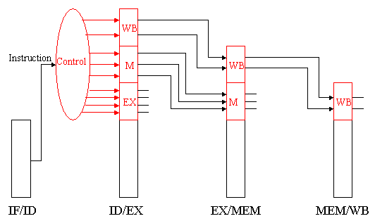
Figure five.5. Propagation of control through the EX, MEM, and WB states of the MIPS pipelined datapath [Maf01,MK98].

Here, the following stages perform piece of work as specified:

• IF/ID: Initializes control by passing the rs, rd, and rt fields of the instruction, together with the opcode and funct fields, to the control circuitry.

• ID/EX: Buffers control for the EX, MEM, and WB stages, while executing control for the EX stage. Control decides what operands volition exist input to the ALU, what ALU operation volition be performed, and whether or non a co-operative is to be taken based on the ALU Zero output.

• EX/MEM: Buffers control for the MEM and WB stages, while executing control for the MEM stage. The control lines are set for retentivity read or write, equally well as for data selection for retentivity write. This phase of command also contains the branch command logic.

• MEM/WB: Buffers and executes control for the WB stage, and selects the value to exist written into the register file.

Effigy 5.6 shows how the command lines (red) are arranged on a per-stage basis, and how the stage-specific command signals are buffered and passed along to the side by side applicative stage.

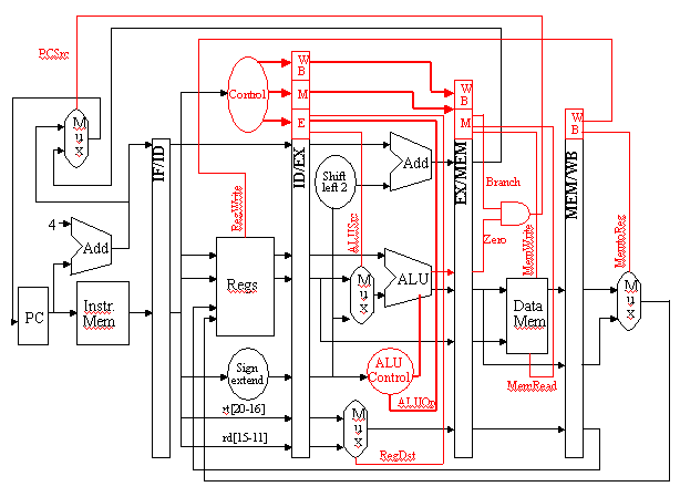
Effigy 5.6. Propagation of command through the EX, MEM, and WB states of the MIPS pipelined datapath [Maf01,MK98].

Reading Assigment: Report the propagation of control signals for the example plan given on p. 471 of the textbook, which is illustrated stepwise on pp. 472-476 of the textbook.

v.3.two. Overview of Hazards

Pipeline processors have several problems associated with controlling smooth, efficient execution of instructions on the pipeline. These problems are more often than not chosen hazards, and include the post-obit 3 types:

• Structural Hazards occur when different instructions collide while trying to access the aforementioned slice of hardware in the same segment of a pipeline. This type of gamble tin can exist alleviated by having redundant hardware for the segments wherein the standoff occurs. Occasionally, it is possible to insert stalls or reorder instructions to omit this blazon of hazard.

• Data Hazards occur when an instruction depends on the effect of a previous education still in the pipeline, which effect has not yet been computed. The simplest remedy inserts stalls in the execution sequence, which reduces the pipeline'due south efficiency. The solution to information dependencies is twofold. Commencement, one can frontwards the ALU result to the writeback or data fetch stages. 2d, in selected instances, information technology is possible to restructure the code to eliminate some information dependencies. Forwarding paths are shown as thin blue or red lines in Figure v.iv.

• Control Hazards can result from branch instructions. Here, the branch target address might not be ready in time for the branch to be taken, which results in stalls (dead segments) in the pipeline that accept to be inserted as local await events, until processing can resume later on the branch target is executed. Command hazards can be mitigated through accurate branch prediction (which is difficult), and by delayed branch strategies.

We next examine hazards in detail, and talk over several techniques for eliminating or relieving hazards.

5.three.3. Data Hazards

Definition. A information run a risk occurs when the electric current instruction requires the result of a preceding instruction, merely at that place are insufficient segments in the pipeline to compute the result and write it back to the register file in time for the current instruction to read that upshot from the annals file.

We typically remedy this problem in one of 3 ways:

• Forwarding: In order to resolve a dependency, i adds special circuitry to the pipeline that is comprised of wires and switches with which one forwards or transmits the desired value to the pipeline segment that needs that value for ciphering. Although this adds hardware and command circuitry, the method works considering information technology takes far less fourth dimension for the required value(s) to travel through a wire than it does for a pipeline segment to compute its result.

• Lawmaking Re-Ordering: Here, the compiler reorders statements in the source code, or the assembler reorders object code, to place one or more than statements between the current teaching and the didactics in which the required operand was computed as a result. This requires an "intelligent" compiler or assembler, which must take detailed information almost the structure and timing of the pipeline on which the information hazard would occur. We call this blazon of software a hardware-dependent compiler.

• Stall Insertion: Information technology is possible to insert ane or more stalls (no-op instructions) into the pipeline, which delays the execution of the current teaching until the required operand is written to the register file. This decreases pipeline efficiency and throughput, which is contrary to the goals of pipeline processor design. Stalls are an expedient method of last resort that can be used when compiler action or forwarding fails or might non be supported in hardware or software design.

  The post-obit example is illustrative.

  Example. Suppose nosotros have the following sequence of instructions:

                  sub   $2,   $1,   $3   # Register two is the output of sub      and   $8,   $2,   $5   # Operand #ane depends on Register 2 data      or    $nine,   $six,   $two   # Operand #2 depends on Annals 2 data      add   $7,   $ii,   $two   # Add result depends on Annals 2 data      sw    $6,xx($two)        # Store (retentivity write) depends on Register ii              

  whose pipeline scheduling diagram is shown in Figure 5.seven.

  

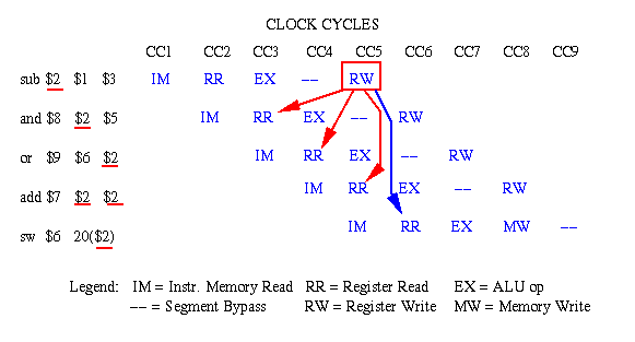
  Effigy five.7. Case of data hazards in a sequence of MIPS instructions, where the red (blueish) arrows indicate dependencies that are problematic (not problematic) [Pat98,MK98].

  Trouble: The beginning instruction (sub), starting on clock cycle 1 (CC1) completes on CC5, when the outcome in Register 2 is written to the register file. If we did nothing to resolve information dependencies, then no didactics that read Register 2 from the register file could read the "new" value computed by the sub instruction until CC5. The dependencies in the other instructions are illustrated past solid lines with arrowheads. If register read and write cannot occur within the aforementioned clock cycle (we will see how this could happen in Section 5.3.iv), then just the fifth instruction (sw) can access the contents of register two in the style indicated by the flow of sequential execution in the MIPS code fragment shown previously.

  Solution #1 - Forwarding: The result generated by the sub instruction can be forwarded to the other stages of the pipeline using special command circuitry (data double-decker switchable to whatever other segment, which can exist implemented via a decoder or batten switch). This is indicated notionally in Figure 5.vii past solid blood-red lines with arrowheads. If the register file can read in the first half of a cycle and write in the second half of a cycle, then the forwarding in CC5 is not problematic. Otherwise, we would have to delay the execution of the add together educational activity by one clock bike (encounter Figure 5.9 for insertion of a stall).

  Solution #2 - Code Re-Ordering: Since all Instructions two through v in the MIPS code fragment crave Register 2 as an operand, nosotros do not have instructions in that particular code fragment to put between Instruction 1 and Instruction 2. However, allow us presume that we have other instructions that (a) do not depend on the results of Instructions i-5, and (b) themselves induce no dependencies in Instructions one-5 (e.thousand., by writing to register one, 2, 3, five, or half-dozen). In that example, nosotros could insert 2 instructions betwixt Instructions 1 and 2, if register read and write could occur concurrently. Otherwise, we would have to insert three such instructions. The latter case is illustrated in the following effigy, where the inserted instructions and their pipeline actions are colored dark green.

  

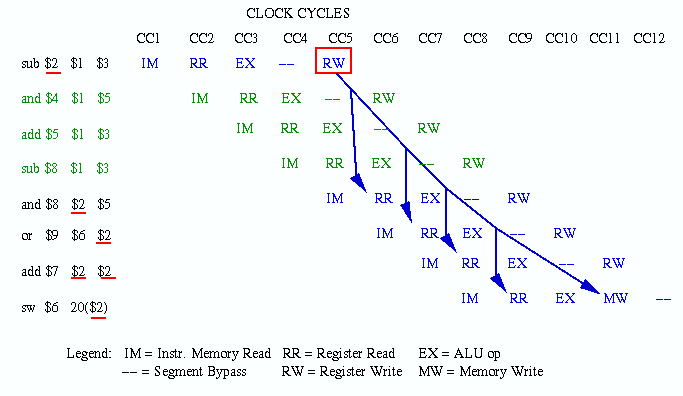
  Figure five.8. Example of code reordering to solve data hazards in a sequence of MIPS instructions [Pat98,MK98].

  Solution #three - Stalls: Suppose that we had no instructions to insert between Instructions 1 and 2. For example, there might be data dependencies arising from the inserted instructions that would themselves accept to be repaired. Alternatively, the programme execution lodge (functional dependencies) might not allow the reordering of code. In such cases, we have to insert stalls, also chosen bubbles, which are no-op instructions that only delay the pipeline execution until the dependencies are no longer problematic with respect to pipeline timing. This is illustrated in Figure 5.9 by inserting three stalls betwixt Instructions 1 and two.

  

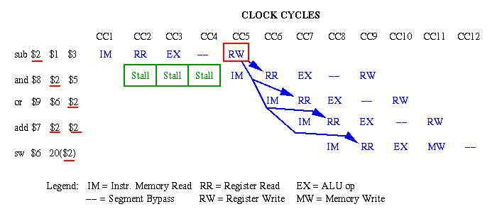
  Effigy v.nine. Example of stall insertion to solve information hazards in a sequence of MIPS instructions [Pat98,MK98].

  As mentioned previously, the insertion of stalls is the least desireable technique because information technology delays the execution of an instruction without accomplishing any useful piece of work (in contrast to lawmaking re-ordering).

  five.3.4. Structural Hazards

  Definition. A structural hazard occurs when in that location is insufficient hardware to support a ciphering in a given pipeline segment.

  For example, consider the data dependency betwixt the outset and fourth instructions (sub and add) of the example in Department 5.3.3. Here, a register file write and a register file read are scheduled in CC5. This tin be resolved by (a) duplicating hardware, or (b) modifying the existing hardware to support concurrent operations. If we duplicated the register file, then we could perform concurrent read and write operations, but at that place would exist a consistency problem. That is, at a given clock cycle, registers in one register file could accept different values than the corresponding registers in the other annals file. This inconsistency is clearly unacceptable if accurate computation is to exist maintained.

  Instead, we tin can alter the annals file so that it (1) performs register write on the kickoff half of the clock cycle and (2) performs register read on the second one-half of the clock bicycle. In earlier hardware, designers sometimes inserted a delay between write and read that was very minor in relation to the clock cycle time, in order to ensure convergence of the register file write.

  Other structural hazards could occur during the branch instruction, if there were not two ALUs in the EX segment of the pipeline. That is, with only 1 ALU, nosotros would have to simultaneously compute the BTA and decide (via subtraction) whether or non the co-operative condition was fulfilled. This would non be possible without ii concurrent adders in the ALU, which is what nosotros currently have in our MIPS pipeline pattern shown in Figure v.4.

  A farther structural hazard could occur if we simply used one memory for both instructions and data. For instance, in Effigy 5.7, suppose the sub instruction was instead a sw instruction. Then, nosotros would be writing to data memory in CC4 for Didactics #1 and reading from didactics memory in CC4 for Instruction #iv. Clearly, if at that place was just one memory in that location would be a conflict.

  Similar to the problem with the concurrent reads and writes on the register file, there are two ways to solve this dilemma. First, we tin can blueprint a special-purpose retention module that permits writing (reading) on the first (resp. second) half of the clock cycle, as we said could be done with the annals file. Withal, this requires special (expensive) hardware. Second, nosotros can utilise ii fast caches, 1 for instructions, and ane for data, that access a large, slower main memory in which instructions and data are both stored. The latter method is used in practice because caches and main memory already exist, and the retentiveness management hardware for these types of components too exists. Thus, we can use off-the-shelf hardware to solve a problem that would otherwise crave special-purpose development of expensive hardware. Although this might not be as much fun as developing new hardware, it is more price-effective, which matters when ane is designing and producing computers for profit.

  5.3.v. Control (Branch) Hazards

  Control hazards are the near difficult types of hazards arising from normal operation of a program. In the next section, we will see that exceptions (e.yard., overflow) can play especially interesting types of havoc with polish pipeline execution.

  The about common type of control take a chance is the co-operative education, which has two alternative results: (1) bound to the branch target address if the pedagogy succeeds, or (2) execute the instruction after the branch (at PC+4 of instruction memory) if the branch fails.

  The trouble with the branch instruction is that we usually exercise non know which event will occur (i.eastward., whether or not the branch will exist taken) until the branch condition is computed. Frequently, the co-operative status depends on the upshot of the preceding instruction, so we cannot precompute the branch condition to discover out whether or not the branch will exist taken.

  The following four strategies are employed in resolving control dependencies due to branch instructions.

  5.3.5.1. Assume Branch Not Taken. As we saw previously, we can insert stalls until we find out whether or non the branch is taken. Still, this slows pipeline execution unacceptably. A common alternative to stalling is to continue execution of the educational activity stream as though the branch was non taken. The intervening instructions betwixt the branch and its target are then executed. If the branch is non taken, this is not a harmful or confusing technique. However, if the branch is taken, and so we must discard the results of the instructions executed afterwards the branch statement. This is done by flushing the IF, ID, and EX stages of the pipeline for the discarded instructions. Execution continues uninterrupted after the branch target.

  The cost of this technique is approximately equal to the price of discarding instructions. For instance, if branches are non taken 50 percent of the time, and the toll of discarding results is negligible, then this technique reduces by l percent the toll of control hazards.

  5.3.five.2. Reducing Branch Delay. In the MIPS pipeline architecture shown schematically in Figure 5.4, we currently assume that the co-operative condition is evaluated in Stage 3 of the pipeline (EX). If nosotros motility the branch evaluation up one stage, and put special circuitry in the ID (Decode, Stage #2), then we tin can evaluate the co-operative condition for the beq instruction. This would allow united states to take the branch in EX instead of MEM, since we would accept ready for Stage 3 (EX) the Zero output of the comparator that would normally exist computed in EX. The hardware needed to compute equality is just a serial of parallel xnor gates and-ed together, then inverted.

  Exercise: Determine how this type of circuitry could be configured.

  The advantage of this technique is that only i instruction needs to be discarded rather than two, as in the previous department. This reduces hardware price and time required to flush the pipeline, since just the IF and ID stages would need to be flushed, instead of the iii stages in the preceding case.

  5.3.5.3. Dynamic Branch Prediction. It would exist useful to be able to predict whether or not a majority of the branches are taken or non taken. This tin exist done in software, using intelligent compilers, and can as well be done at runtime. Nosotros concentrate on the software-intensive techniques first, since they are less expensive to implement (being closer to the compiler, which is easier to modify than the hardware).

  The most advantageous situation is i where the branch condition does non depend on instructions immemdiately preceding it, as shown in the following code fragment:

                add $five, $5, $6     # One of the registers for beq comparing is modified      sub $four, $3, $6     # Goose egg important to the branch here      and $vii, $eight, $half dozen     # Nix important to the branch here      and $9, $6, $6     # Nothing important to the branch here                              beq $5, $6,              target            

  Here, the branch compares Registers 5 and 6, which are final modified in the add instruction. We tin can therefore precompute the branch status as sub r $5, $6, where r denotes a destination register. If r = 0, then we know the co-operative will be taken, and the runtime module (pipeline loader) tin schedule the jump to the co-operative target address with full conviction that the branch will exist taken.

  Another approach is to continue a history of branch statements, and to tape what addresses these statements branch. Since the vast bulk of branches are used as tests of loop indices, then we know that the branch will virtually always spring to the loopback point. If the branch fails, then we know the loop is finished, and this happens simply once per loop. Since most loops are designed to have many iterations, branch failure occurs less frequently in loops than does taking the branch.

  Thus, information technology makes good sense to presume that a branch will bound to the place that it jumped to before. However, in dense decision structures (e.g., nested or cascaded if statements), this situation does not ever occur. In such cases, ane might non be able to tell from the preceding branch whether or not the branching behavior will be repeated. Information technology is and so reasonable to use a multi-branch lookahead.

  Reading Assigment: Written report the discussion of multi-fleck branch prediction schemes given on pp. 501-502 of the textbook.

  Another clever technique of making branches more than efficient is the branch delay slot. Nosotros previously discussed delayed branches when we overviewed the multicycle datapath implementation of the beq pedagogy. In summary, the concept of efficient branching has two parts. First, the co-operative target address is computed in the ID stage of the pipeline, to decide equally early as possible the didactics to fetch if the co-operative succeeds. Since this is done in the second phase of the pipeline, at that place is an instruction I following this (in the commencement or IF phase). Later I moves to the ID stage, then the branch target (pointed to by either PC+4 or the BTA) is loaded into the IF stage.

  It is this instruction (I) that is called the co-operative delay slot (BDS). In the BDS tin be safely placed an instruction that does not accept data dependencies with respect to (a) the branch condition, (b) the instruction following the branch status, or (c) the branch target. This ensures that, when the education J is executed (J is the instruction to which command is transferred later the branch condition is evaluated, whether J is pointed to past PC+4 or BTA), then the instruction I will have been executed previously, and the piping will not accept a stall where I would have been. Equally a upshot, the pipe will remain total throughout the branch evaluation and execution, unless an exception occurs.

  5.iii.half-dozen. Exceptions as Hazards

  Hardware and software must work together in any architecture, especially in a pipeline processor. Here, the ISA and processor control must be designed so that the following steps occur when an exception is detected:

  1. Hardware detects an exception (east.g., overflow in the ALU) and stops the offending instruction at the EX stage.

  2. Pipeline loader and scheduler allow all prior instructions (e.g., those already in the pipeline in MEM and WB) to complete.

  3. All instructions that are present in the pipeline afterward the exception is detected are flushed from the pipeline.

  4. The address of the offending pedagogy (unremarkably the address in primary memory) is saved in the EPC register, and a code describing the exception is saved in the Cause annals.

  5. Hardware control branches to the exception handling routine (part of the operating system).

  6. The exception handler performs ane of three actions: (i) notify the user of the exception (e.g., dissever-by-zero or arithmetic-overflow) then terminate the program; (2) try to correct or mitigate the exception and then restart the offending instruction; or (iii) if the exception is a benign interrupt (e.g., an I/O request), then salve the programme/pipeline land, service the interrupt request, and so restart the plan at the instruction pointed to by EPC + 4.

  In whatsoever case, the pipeline is flushed every bit described.

  In general, we tin say that, if a pipeline has N segments, and the EX stage is at segment i < i < Northward, then ii observations are key to the prediction of pipeline performance:

  • Flushing negates the processing of the (i-1) instructions following the offending instruction. These must be reloaded into the pipe, at the price of i cycles (one bicycle to flush, i-1 cycles to reload the i-i instructions after the exception is processed).

  • Completing the N-i instructions that were loaded into the pipeline prior to the offending didactics takes N-i clock cycles, which are executed (a) prior to, or (b) concurrently with, the reloading of the instructions i-1 that followed the i-th instruction (in the EX stage).

  Information technology is readily seen that the total number of wasted cycles equals (i-1) + (N-i) = N - 1, which is precisely the number of cycles that it takes to ready up or reload the pipeline.

  The proliferation of unproductive cycles tin be mitigated past the following technique:

  1. Freeze the pipeline country as presently equally an exception is detected.

  2. Procedure the exception via the exception handler, and decide whether or not to halt or restart the pipeline.

  3. If the pipeline is restarted, reload the (i-i) instructions post-obit the offending educational activity, concurrently with completing execution of the (Due north-i) instructions that were existence processed prior to the offending education.

  If Step 3 tin can be performed as stated, then the all-time-case penalisation is just i bike, plus the time incurred by executing the exception handler. If the unabridged pipeline needs to be flushed and restarted, then the worst-case penalization is North cycles incurred by flushing the pipe, then reloading the pipeline after the instructions preceding the offending instruction accept been executed. If the offending educational activity must be restarted, then a maximum of i cycles are lost (one cycle for flush, plus (i-1) cycles to restart the instructions in the pipe post-obit the offending teaching).

  In the adjacent department, we collect the concepts about pipeline operation that nosotros have been discussing, and show how to compute the CPI for a pipeline processor under constraint of stalls, structural hazards, branch penalties, and exception penalties.

  5.four. Pipeline Performance Analysis

  Reading Assignments and Exercises

  Equally we said early on in this grade, we are trying to teach the technique of performance analysis, which helps one to intelligently determine whether or not a given processor is suitable computationally for a specific application. In this section, we develop performance equations for a pipeline processor, and do so in a stepwise way, so yous can see how the diverse hazards and penalties affect operation.

  5.4.1. CPI of a Pipeline Processor

  Suppose an North-segment pipeline processes M instructions without stalls or penalties. We know that it takes Due north-i cycles to load (setup) the pipeline, and M cycles to complete the instructions. Thus, the number of cycles is given by:

  N_cyc = N + K - 1 .

  The cycles per education are easily computed:

  CPI = North_cyc/M = ane + (N - i)/Thousand .

  Thus, CPI for a finite program volition always be greater than one. This stands in sharp contradiction to the starting time fallacy of pipeline processing, which says:

  Fallacy #i: CPI of a pipeline processor is always equal to 1.0, since ane instruction is processed per bicycle.

  This argument is beguiling because it ignores the overhead that we take just discussed. The fallacy is like to claiming that you only spend eight hours at the office each twenty-four hour period, so you must have 16 hours per day of "fun fourth dimension". Still, you accept to take fourth dimension to commute to/from the office, buy groceries, and practice all the other homely tasks of life, many of which are in no fashion related to "fun time". In exercise, such tasks are drudgery that is a type of overhead.

  5.4.2. Issue of Stalls

  Now let usa add together some stalls to the pipeline processing scheme. Suppose that nosotros take a N-segment pipeline processing Thousand instructions, and we must insert K stalls to resolve information dependencies. This ways that the pipeline now has a setup penalization of Northward-1 cycles, every bit earlier, a stall punishment of K cycles, and a processing cost (as before) of Grand cycles to process the Chiliad instructions. Thus, our governing equations get:

  N_cyc = N + Yard + K - 1 .

  and

  CPI = N_cyc/M = 1 + (N + K - 1)/M .

  In practice, what does this tell united states? Namely, that the stall penalisation (and all the other penalties that nosotros will examine) adversely touch on CPI. Here is an instance to testify how we would analyze the problem of stalls in a pipelined plan where the percentage of instructions that incur stalls versus not-stalls are specified.

  Example. Suppose that an N-segment pipeline executes M instructions, and that a fraction f_stall of the instructions require the insertion of K stalls per instruction to resolve data dependencies. The total number of stalls is given by f_stall · M · Chiliad (fraction of instructions that are stalls, times the full number of instructions, times the boilerplate number of stalls per educational activity). By substitution, our preceding equations for pipeline performance become:

  North_cyc = Northward + One thousand + (f_stall · One thousand · K) - i .

  and

  CPI = Due north_cyc/1000 = one + (f_stall · Yard) + (Due north - 1)/M .

  And so, the CPI penalisation due to the combined effects of setup toll and stalls at present increases to fK + (Northward - 1)/Thou. If f_stall = 0.1, K = iii, N = v, and Thou = 100, then CPI = i + 0.three + 4/100 = i.34, which is 34 per centum larger than the fallacious assumption of CPI = one.

  This leads to the adjacent fallacy of pipeline processing:

  Fallacy #two: Stalls are not a big problem with pipelines - y'all only accept to worry near the number of stalls, not the percentage of instructions that induce stalls.

  This fallacy is particularly dangerous. It is analogous to saying that the only thing that matters is the number of home burglaries each year, not the burglary rate per capita. If y'all move to a new neighborhood, you desire to know both the number and per-capita incidence of crimes in that neighborhood, not merely the robbery count. Then you can make up one's mind, from the population, whether or not it is safe to live in that location.

  Similarly, with a pipeline processor, you want to determine whether or non the didactics mix or ordering of instructions causes data dependencies, and what is the incidence of such dependencies. For example, 1,000 instruction program with 20 stalls will run more than efficiently than a ane,000 teaching program with xx percent of the instructions requiring one stall each to resolve dependencies.

  five.4.3. Effect of Exceptions

  For purposes of discussion, assume that we have Chiliad instructions executing on an N-segment pipeline with no stalls, only that a fraction f_ex of the instructions raise an exception in the EX phase. Further assume that each exception requires that (a) the pipeline segments before the EX phase exist flushed, (b) that the exception be handled, requiring an average of H cycles per exception, so that (c) the educational activity causing the exception and its following instructions be reloaded into the pipeline.

  Thus, f_ex · M instructions will crusade exceptions. In the MIPS pipeline, each of these instructions causes three instructions to be flushed out of the pipe (IF, ID, and EX stages), which incurs a penalty of four cycles (one cycle to flush, and three to reload) plus H cycles to handle the exception. Thus, the pipeline performance equations get:

  N_cyc = N - ane + (1 - f_ex) · M + (f_ex · M · (H + four)) ,

  which we can rewrite as

  N_cyc = Thou + [Northward - 1 - Thou + (1 - f_ex) · 1000 + (f_ex · M · (H + four))] .

  Rearranging terms, the equation for CPI tin can exist expressed as

  CPI = Northward_cyc/M = ane + [1 - f_ex + (f_ex · (H+four)) - ane + (North - 1)/G] .

  Afterwards combining terms, this becomes:

  CPI = N_cyc/M = 1 + [(f_ex · (H+3)) + (N - i)/G] .

  We can come across by test of this equation and the expression for CPI due to stalls that exceptions have a more detrimental upshot, for two reasons. Get-go, the overhead for stalls (One thousand stalls per affected instruction) is K < 4 cycles in the MIPS pipeline (since the pipeline has but five segments). Second, the cost of each exception is H+3 cycles per affected educational activity. Since H > 0 for a nontrivial exception handler, the toll of an exception in the MIPS pipeline (under the preceding assumptions) will exceed the price of remedying a hazard using stalls. The good news, however, is that in that location are usually fewer exceptions in programs than data or structural dependencies, with the exception of I/O-intensive programs (many I/O interrupts) and arithmetic-intensive programs (possible overflow or underflow exceptions).

  5.4.4. Effect of Branches

  Branches present a more complex picture in pipeline performance analysis. Recall that there are iii ways of dealing with a branch: (1) Assume the branch is not taken, and if the co-operative is taken, flush the instructions in the pipe after the branch, then insert the teaching pointed to by the BTA; (2) the converse of 1); and (3) use a delayed branch with a branch delay slot and re-ordering of lawmaking (assuming that this can be done).

  The showtime two cases are symmetric. Assume that an fault in branch prediction (i.eastward., taking the branch when yous expected not to, and conversely) requires L educational activity to be flushed from the pipeline (one cycle for flushing plus L-ane "dead" cycles, since the branch target can exist inserted in the IF stage). Thus, the cost of each branch prediction error is L cycles. Further assume that a fraction f_br of the instructions are branches and f_exist of these instructions outcome in branch prediction errors.

  The penalisation in cycles for branch prediction errors is thus given past

  branch_penalty = f_br · f_be · M instructions · L cycles per instruction .

  The pipeline performance equations then become:

  N_cyc = N - i + (ane - f_br · f_be) · Yard + (f_br · f_be · G · L) ,

  which we can rewrite as

  N_cyc = M + [N - 1 - M + (one - f_br · f_be) · M + (f_br · f_be · M · Fifty) ,

  Rearranging terms, the equation for CPI tin can be expressed as

  CPI = N_cyc/One thousand = i + [(i - f_br · f_be) + (f_br · f_be · L) - 1 + (Due north - 1)/M] .

  Afterwards combining terms, this becomes:

  CPI = Due north_cyc/M = ane + [(f_br · f_be · (L-ane)) + (Due north - 1)/G] .

  In the instance of the branch delay slot, we assume that the branch target address is computed and the co-operative condition is evaluated at the ID stage. Thus, if the branch prediction is correct, there is no penalty. Depending on the method by which the pipeline evaluates the co-operative and fetches (or pre-fetches) the branch target, a maximum of two cycles punishment (one cycle for flushing, one bicycle for fetching and inserting the co-operative target) is incurred for insertion of a stall in the instance of a branch prediction mistake. In this case, the pipeline performance equations become:

  N_cyc = N - 1 + (1 - f_br · f_be) · G + (f_br · f_be · 2M) ,

  which implies the following equation for CPI every bit a role of branches and co-operative prediction errors:

  CPI = Due north_cyc/G = 1 + [f_br · f_be + (Due north - one)/Thousand] .

  Since f_br << ane is usual, and f_be is, on boilerplate, assumed to be no worse than 0.v, the production f_br · f_be, which represents the additional co-operative penalization for CPI in the presence of delayed co-operative and BDS, is generally small.

  ________________//_______________

  This concludes our discussion of pipelining. We adjacent concentrate on the discussion and analysis of supporting technologies, such as memories and buses.

References

[Maf01] Mafla, Due east. Grade Notes, CDA3101, at URL http://www.cise.ufl.edu/~emafla/ (as-of 11 Apr 2001).

[MK98] Copyright 1998 Morgan Kaufmann Publishers, Inc. All Rights Reserved, per copyright observe request at http://www.mkp.com/books_catalog/cod2/cod2ecrt.htm (1998).

[Pat98] Patterson, D.A. and J.L. Hennesey. Estimator Arrangement and Blueprint: The Hardware/Software Interface, Second Edition, San Francisco, CA: Morgan Kaufman (1998).

Reading and Writing Memory in Different Halves of the Cycle

Source: https://www.cise.ufl.edu/~mssz/CompOrg/CDA-pipe.html

Share this post